
This project was created as a course deliverable in Danish University of Technology Deep learning course. The main goal of the project was to get a hends on project with a real world use case where deep learning techniques can be applied.
Deep learning has shown tremendous improvement within computer vision over the last decade. A field that has also been expanding due to recent advances in deep learning is medical image classification. However, there are still a lot to explore in this field in terms of different disease classification and reliability of the algorithms. This project focuses on exploring the potential of deep learning in classifying two skin diseases: Eczema vs. Cutaneus T-celle Lymfoma/Mycosis Fungoides.In the project, different experiments were performed by training a network from scratch, using transfer learning and a spatial transformer.
The data
The original dataset was provided by Alborg university hospital and cointained 10308 images. There were 7131 (70.94% of the dataset) images of Eczema and 2995 (29.06% of the dataset) images of Cutaneus T-celle Lymfoma/Mycosis Fungoides, which meant that there is a class imbalance in our dataset. Another problem we faced during research was very variant images.
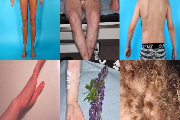
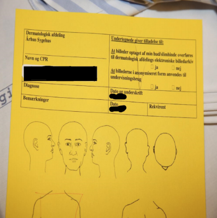
As shown in the picture above, all of the images contains different parts of the body. In some of the pictures it was very hard, even for a human eye, to notice an effected area of the disease. In others, we observed an outside objects, which clearly made our classification more difficult. We also performed few preprocessing steps like filtering out patient’s journal images using K-means classification.
We also resized all images as the original 4000x4000 resolution was way too big. All the images were normalized per channel either to have the center to the mean and unit variance or using min-max normalization. Experimentation showed that the choice of which normalization technique to use did not play a role in the outcome.
Modeling
Before experimentation, we first developed an overall plan of attack. One of the main challenges with this dataset is the size of the images. State of the art networks usually do not go beyond 300x300 pixels, and our data had over 4000x4000 pixels in size. In order to overcome this challenge, the idea was to adapt the spatial transformer from to crop the original images and then apply a classifier on the cropped image. Figure shows the overall idea.
First the original image would be resized, and its new version fed into the localization network, which calculates theta. Then, the transformation grid and sampler would use theta to apply the transformation on the original image. The intuition is that the localization would learn where to zoom in to find the disease affected area and the actual zooming would be done in the original image, preserving the full resolution. The final cropped image would then be passed to the classifier network.

Experiments
Finding the correct architecture and tunning hyper-parameters is never a problem that is fully solved. Starting with a very complex network can lead to difficult reasoning behind what went wrong. Moreover, experimentation with smaller networks are faster and allow for quicker insights. Thus, we opted to start small and test ideas as independently as possible.
Custom CNN
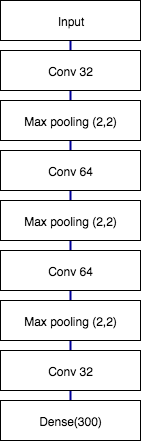
The first approach was to create a more complex architecture. We’ve based ourselves on the VGG architecture in order to do so, the network is shown in picture below. Each block is composed of two convolutional layers followed by a max pooling layer. Padding is done so the input size is preserved for every convolution. The kernel size is always 3 by 3 while max pooling is done 2 by 2. All the activations are relu, except from the last two neurons, which are softmax. The loss function used was also crossentropy.

Transfer learning
The second approach was to try and use a pre-trained network on top of the resized images. We choose VGG as it has a less complex network than other state-of-the-art, being more intuitive to work with. For all the experiments, the last fully connected layers were substituted with the same structure as the fully connected layers in and weights reinitialized. two different experiments were performed:
- Freezing the first 11 layers and training the remaining with a learning rate 10 times smaller.
- Freezing the first 14 layers and training the remaining with a learning rate 10 times smaller.
The first experiment freezes all convolutional layers up to the third stack of convolutions, and fine tune all the layers that follow. The second experiment does the same, but with fine tunning only higher level features. Both experiments cutting points are illustrated in picture below.

Spatial transformer
At first, we began our experiments with spatial transformer on famous MNIST dataset. This was done to test the performance of the model on a small and simple dataset and make sure our code work. For our localisation network, we used the following structure shown in picture below.
For the classification after spatial transformer we used custom CNN model. After successful try on MNIST we tried to implement the same spatial transformer both to custom CNN with dermatology dataset and to transfer learning.
Data augmentation
At the end of our project we also came up with idea to test dataset augmentation, because sometimes this can improve results quite drastically.
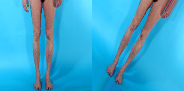
Firstly, as we are dealing with dermatology diseases which both have red hue, overexposing the images could help the classification task. With this technique the skin becomes almost white, while the disease region increase in color. To achieve this library was used providing us with adaptive histogram equalization which enhanced the details and increased image exposure. The result is shown in figure.

Secondly, we also experimented using some transformations that could increase the classifier robustness. The augmentation was done randomly for each transformation in a given range at each epoch. An example of a transformed image is shown in the picture. The following transformations were used:
- rotation: random rotations of up to 40 degrees
- width and height translation : random horizontal and vertical translations of up to 20% of the total width.
- Shear transformation: up to 0.2 shear angle in counter-clockwise direction as radians
- zoom: randomly zooming on up to 20%
So how about the results?
In this project we have created a model that distinguishes 80% of the times correctly between Eczema vs. Cutaneus T-celle Lymfoma/Mycosis Fungoides diseases. Moreover, the model classifies correctly cases of Cutaneus T-celle Lymfoma/Mycosis Fungoides more often than Eczema. Given the accuracy achieved that is still a modest result, it is a significant improvement over the base model of 68%. Overfitting was the biggest challenged faced across experiments. We attribute overfitting to two main causes: non-relevant pixels on the original image and dataset size. Furthermore, transfer learning coupled with data augmentation proved to be the best techniques to face this issue. Another challenge was to locate the disease affect area in the image in order to avoid noise pixels. Unfortunately, doing so using a spatial transformer did not work. We believe that this can be due to a very complex dataset with heterogeneous noise and/or the localisation network being too simple.